
Tutorial · Intermediate · 14 min read
Detecting Line Maze Junctions With an IR Array
How a line follower tells a T junction from a cross, a dead end from the finish—and why one sensor reading is never enough to decide.
A line follower has one job: keep the line centred. A line maze robot has two, and the second one is where beginners get stuck. It must still follow the line, but it must also notice the moments when the line offers a choice—and decide what kind of choice it is.
That decision layer sits on top of the PID loop, not inside it. The controller should never know what a maze is. It steers toward a line; the junction layer watches the same sensor readings for the patterns that mean “something changed” and takes over when one appears.
Six things a junction can be
Every junction in a taped line maze reduces to one of six cases. With an 8-channel reflectance array reading 1 for black tape and 0 for the white board, each produces a signature:
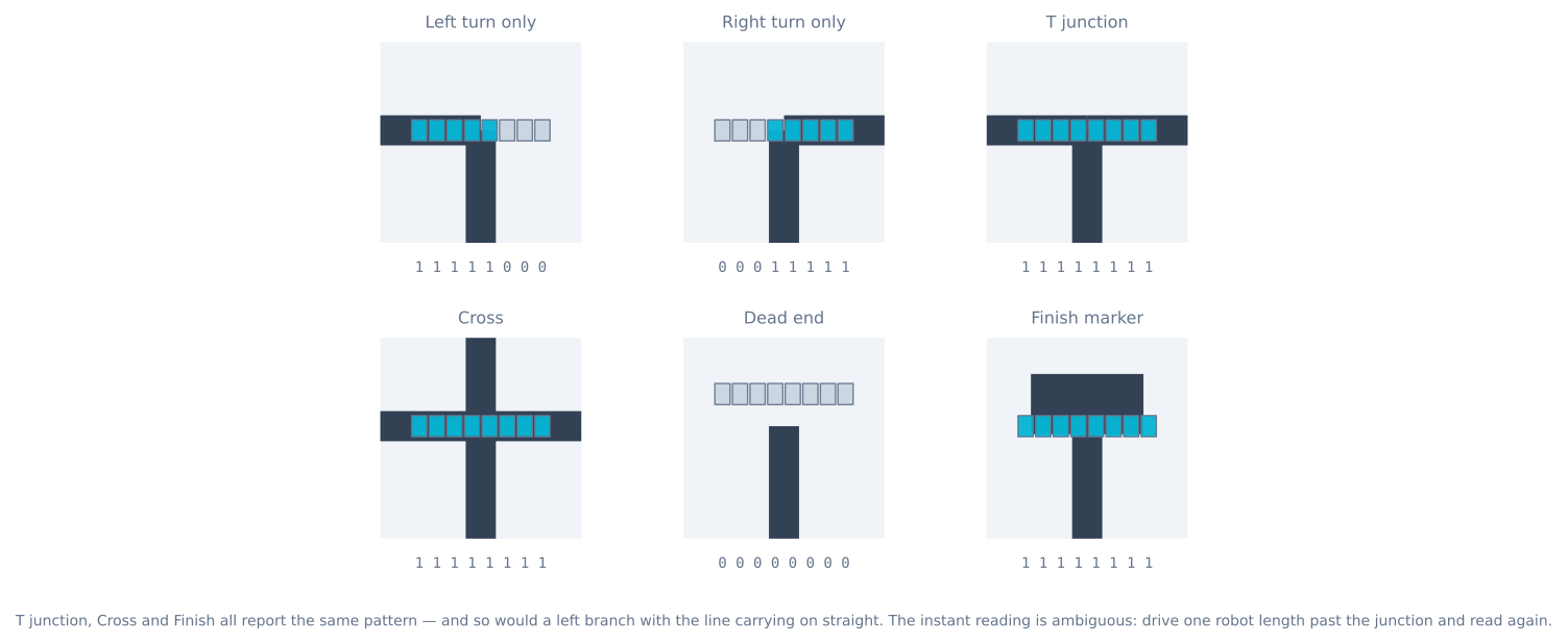
- Left turn only — the outer left sensors go black while the right side stays white.
- Right turn only — the mirror image.
- T junction — tape spans the full width, with nothing ahead.
- Cross — tape spans the full width, and the line continues ahead.
- Dead end — every sensor reads white; the line simply stopped.
- Finish — a solid filled block, wide and long, that stays black as you drive into it.
The reading alone is ambiguous
Look at the T junction, the cross, and the finish marker. All three report 11111111. A left branch where the line also continues straight reports the same thing as a plain left turn.
This is the part worth internalising: the instantaneous sensor pattern cannot classify a junction. A robot that decides the moment its outer sensors go black will confidently turn left at a crossroads it should have driven straight through.
The fix is motion, not more sensors. When the array first reports a wide black pattern:
- Record which side (or sides) went black—that is the set of available branches.
- Keep driving forward by roughly one robot length.
- Read again. If the centre sensors still see tape, straight ahead was also an option. If everything is white, it was a T. If everything is still black, you have driven into the finish block.
Only now do you know what kind of junction you left behind, and only now can the maze layer choose.
Junction classify(Sensors& s) {
  Branches at = s.readWideBranches();      // left / right seen on arrival
  driveForward(ONE_ROBOT_LENGTH);          // commit past the intersection
  Reading after = s.read();

  if (after.allBlack())  return FINISH;    // still on tape = solid block
  at.straight = after.centreOnLine();      // line continued through
  return at.toJunction();
}
Note that the classifier drives. That is unusual for a sensing function and it is the point—junction type is a property of a short trajectory, not of a single sample.
Choosing a branch
Once a junction is classified, the maze layer picks a branch by a fixed rule. The left-hand rule—always take the leftmost available branch, and turn back at a dead end—is the standard choice because it is stateless, exhaustive on a maze without loops, and trivial to verify by hand.
Consistency matters more than cleverness here. A robot that always prefers left will eventually visit every reachable branch, and the record of its turns is what the route simplification step later collapses into the optimal path. Watch the same explore-then-optimise behaviour run in the Maze Solver Simulator—that one senses walls rather than tape, but the decision layer above the sensing is identical.
The array has to be wider than the line
Junction detection asks a specific question of the sensor: have the outermost channels gone black while the centre is still on the line? An array barely wider than the tape physically cannot answer it.
   left branch                    8-channel array, ~60 mm wide
   ────────────────┐          [ 1 1 1 0 0 0 0 0 ]   outer left black -> a branch exists
                   │
   ════════════════╪═══════   [ 0 0 0 1 1 0 0 0 ]   centre still on the line
│| Tape width | Minimum useful array width | Why |
|---|---|---|
| 19 mm (standard) | ~60 mm | Outer sensors must clear the tape by a full sensor spacing |
| 25 mm | ~75 mm | |
| 12 mm | ~40 mm |
The rule of thumb is three times the tape width. Narrower and the robot cannot distinguish “the line curved sharply” from “the line branched” — which is the central decision the whole project rests on. An 8-channel array at 8 mm spacing gives about 60 mm, which is why that is the standard choice for 19 mm tape.
Debouncing a junction
The array crosses a junction over several loop iterations, and each one is a fresh reading. A classifier that fires on the first wide pattern will often fire two or three times for one junction, filling the recorded path with characters that were never real turns.
const uint8_t CONFIRM_SAMPLES = 3;      // consecutive readings that must agree
const unsigned long JUNCTION_DEADTIME_MS = 300;

uint8_t agreeCount = 0;
uint8_t lastPattern = 0;
unsigned long lastJunctionAt = 0;

bool junctionDetected(uint8_t pattern) {
  // Ignore everything for a short while after committing to one.
  if (millis() - lastJunctionAt < JUNCTION_DEADTIME_MS) return false;

  if (pattern == lastPattern) agreeCount++;
  else { lastPattern = pattern; agreeCount = 1; }

  if (agreeCount >= CONFIRM_SAMPLES && isWide(pattern)) {
    lastJunctionAt = millis();
    agreeCount = 0;
    return true;
  }
  return false;
}
Sizing the dead time is a genuine trade-off, and it is worth doing with numbers rather than by feel:
deadtime < (minimum spacing between junctions) / speedAt 0.2 m/s with junctions no closer than 15 cm, that is 750 ms of headroom — so 300 ms is safe. Drive at 0.5 m/s in a maze with 10 cm spacing and the budget drops to 200 ms, which is why exploration runs slowly. This constraint, not the algorithm, is what sets the exploration speed.
The turn itself
Classifying the junction is half the job; executing the turn without losing the line is the other half, and a fixed-angle turn is the wrong way to do it.
| Method | How it ends | Reliability |
|---|---|---|
| Turn for a fixed time | After N milliseconds | Poor — changes with battery voltage and surface |
| Turn a fixed angle on encoders | After N counts | Better, but backlash and slip accumulate |
| Turn until the line is reacquired | When the centre sensors see tape | Best — self-correcting, ends where the line is |
void turnUntilLine(int direction) {
  pivot(direction);
  delay(120);                        // clear the junction's own tape first
  while (!centreOnLine()) {          // then rotate until the new line appears
    if (millis() - startedAt > TURN_TIMEOUT_MS) { stopMotors(); fault(); return; }
  }
  stopMotors();
}
The delay(120) matters. Immediately after starting the turn the centre sensors are still over
the junction’s own tape, so a naive “turn until you see the line” stops instantly and the robot
never turns at all. Clear the junction first, then look.
The timeout matters too: without it, a robot that turns past the branch — because it was travelling too fast, or the branch was mis-detected — spins forever.
The full classification, with straight-ahead resolved
Putting the debounce, the drive-past and the turn together:
Junction classifyAndTurn() {
  const Branches at = readWideBranches();     // left and/or right, on arrival

  driveForward(ONE_ROBOT_LENGTH);             // commit past the intersection
  const Reading after = read();

  if (after.allBlack()) return FINISH;        // still on tape = the solid block

  Junction j;
  j.left     = at.left;
  j.right    = at.right;
  j.straight = after.centreOnLine();          // resolved only by moving

  if (!j.left && !j.right && !j.straight) return DEAD_END;
  return j;
}
The classifier drives, which is unusual for a sensing function and is the whole point: junction type is a property of a short trajectory, not of a single sample. Three of the six cases — T, cross and finish — are indistinguishable at the instant of arrival.
Testing it without a maze
You do not need a maze to verify this layer, and building one before the detection works is a common waste of an evening. Lay out one junction of each type on a board and drive the robot over each in turn, printing the classification:
| Test piece | Expected | Common failure |
|---|---|---|
| Plain straight line | No junction at all | Fires on a slight curve — outer threshold too sensitive |
| Gentle curve, 15 cm radius | No junction | Same |
| Left branch only | LEFT |
Detected as T — dead time too short, fired twice |
| Right branch only | RIGHT |
Mirror of the above |
| T junction | T |
Detected as LEFT — did not drive past to resolve straight |
| Cross | CROSS |
Detected as T — the drive-past distance was too short |
| Dead end | DEAD_END |
Detected as line loss and the robot drove on |
| Solid finish block | FINISH |
Detected as CROSS — the block is longer than a junction |
The gentle curve test is the one that catches the most bugs, and it is the one nobody thinks to run. A tight curve momentarily puts several outer sensors on the tape, which looks exactly like a branch. If your robot invents junctions on curves, the fix is to require the outer sensors to stay black over a minimum distance, not just a minimum count of samples — a curve releases them again quickly, a real branch does not.
Troubleshooting
| Symptom | Likely cause | Fix |
|---|---|---|
| Junctions detected on curves | Outer threshold too sensitive | Require the pattern to persist over a minimum distance |
| One junction recorded twice | No dead time | 200–300 ms after committing to a junction |
| T reported as a left turn | Did not drive past to resolve straight ahead | The classifier must move before deciding |
| Cross reported as T | Drive-past distance too short | One full robot length past the intersection |
| Finish reported as cross | The block is longer than a junction | Keep driving; it stays black, a cross does not |
| Junctions missed entirely | Too fast, or the array is too narrow | Slow the explore run; array ≥ 3× the tape width |
| Turns overshoot past the new line | Fixed-time or fixed-angle turn | Turn until the centre sensors reacquire |
| Robot spins forever after a junction | No turn timeout | Add one, and fault cleanly |
| Never turns at all | Reading the junction’s own tape as the new line | Clear the junction before looking |
| Works on one board, not another | Calibration, or ambient light | Recalibrate every power-up; emitter-off subtraction |
Getting it reliable on real tape
Three things break junction detection on hardware far more often than the algorithm does:
- Calibration drift. Run the array’s calibration sweep over both black tape and white board every time you power up, and re-run it when you move to a different room. Ambient infrared from sunlight and fluorescent lights changes the readings.
- Sensor height. 5–8 mm above the floor. Too high and the contrast collapses; too low and a slightly warped board scrapes the array.
- Tape quality. Use 18–20 mm tape and make the junctions physically clean. A frayed corner reads as an intermittent branch, and no amount of code fixes tape that lies to you.
Get plain line following stable on a simple oval first—tune it in the Line Follower Simulator, then on real tape. A maze will hide mechanical and sensor problems behind what looks like a logic bug.
Explore the graph
Part of these builds
Projects and learning paths that include this tutorial.
Further reading