
Line Follower Simulator: Tune a Robot in Your Browser
Build a virtual line-following robot, visualize its sensors, and tune a PID controller with an interactive browser-based robotics simulator.
- Category
- Arduino
- Time
- 45–90 min
- Platform
- Browser · Arduino
01 / Start here
Introduction
A line-following robot turns sensor readings into steering corrections. This project lets you draw a track, change the robot and sensor geometry, then watch a deterministic PID controller respond in real time. Use it to connect control theory with the behavior you would see from an Arduino robot on a physical course.
Live lab / Deterministic 60 Hz model
Line follower simulator
Run the starter track, tune the controller, or pause and draw a course of your own.
Bright nodes are sensors currently detecting the track. The lavender heading line shows steering output. Drawing pauses the robot automatically.
- Elapsed
- 0.0 s
- Distance
- 0 units
- Line error
- 0.000
- Steering
- 0.000
- Track contact
- 100%
Keyboard: focus the course, then use Space to run/pause, N to step, R to reset, D to draw, and F for full screen.
Controls
Use the track presets to establish a baseline, or pause the run and draw directly on the course. Robot speed controls how far the chassis advances per update. Sensor count and spacing change the field of view. The P, I, and D controls change steering response; Step advances one deterministic update while paused.
Start with a moderate speed, five sensors, and the default gains. Change one variable at a time and compare the error, lap time, and time-on-track metrics.
Theory
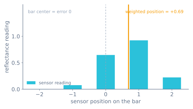
The sensor bar samples reflectance across the front of the robot. Each active sensor contributes its signed position to a weighted average. The center of the bar is error zero; readings left or right of center produce negative or positive error.
The controller combines three terms:
$$u(t) = K_p e(t) + K_i \int e(t)dt + K_d \frac{de(t)}{dt}$$
The correction $u(t)$ speeds one wheel and slows the other. Proportional control reacts to the current offset, integral control corrects persistent bias, and derivative control damps rapid changes.
Algorithm
- Sample every sensor at a fixed interval.
- Compute a weighted line position and normalize it around the center.
- Reuse the last observed line direction when every sensor loses the track.
- Update integral and derivative terms using the same fixed time step.
- Clamp the correction, calculate left and right motor commands, and integrate the robot pose.
Tune proportional gain until the robot follows gentle turns, add derivative gain until oscillation settles, and introduce only enough integral gain to remove a repeatable offset.
Source code
The browser simulator and a microcontroller use the same control shape. A compact Arduino-style loop looks like this:
float integral = 0.0f;
float previousError = 0.0f;

void controlStep(float dt) {
  float error = readWeightedLinePosition();
  integral = constrain(integral + error * dt, -2.0f, 2.0f);
  float derivative = (error - previousError) / dt;
  float correction = kp * error + ki * integral + kd * derivative;

  setMotorSpeeds(baseSpeed - correction, baseSpeed + correction);
  previousError = error;
}
Keep the real control interval stable. A variable delay changes the derivative and integral terms even when the gains stay the same.
Assumptions and hardware differences
This is a teaching model, not a hardware replica. The track is a flat, high-contrast binary mask with no ambient light variation, so the sensor bar sees perfect black and white — on real tape, room lighting, surface gloss and sensor height change the readings and you must calibrate per the steps in the wiring notes. Timing is ideal: the controller runs at a fixed interval with no delay() jitter, whereas a physical Arduino loop varies with other work and that jitter reshapes the PID response. The chassis is kinematic: wheels never slip, motors respond instantly and the battery never sags. Treat gains found here as a close starting point, then re-tune on the real robot after calibration.
Circuit diagram
Connect the sensor outputs to analog-capable inputs, share ground between every module, and drive motors through an H-bridge rather than from controller pins.
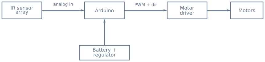
Verify the motor supply rating and add local decoupling near the controller and driver. Never route motor current through a development board’s logic regulator.
Guided experiments
Each of these isolates one variable, which is the thing that is genuinely hard to do on real hardware where everything changes at once.
1. Find the ultimate gain, then halve it
Set the integral and derivative gains to zero and raise the proportional gain until the robot oscillates steadily along a straight section — weaving at a constant amplitude rather than a growing or shrinking one. Halve that value.
You now have a starting Kp derived from a measurement instead of a guess, and it will be
close. Add derivative from there until the weave damps out.
2. Prove that gains are speed-dependent
Tune the robot until it tracks cleanly at a low base speed. Now raise the speed by half and run the same gains without changing anything.
It will weave, cut corners, or lose the line. Nothing about the controller changed — but the same steering correction now produces a larger change in heading per unit of track, so the effective gain went up with the speed. Every tune is a tune at a particular speed, which is why a competition robot slows for corners rather than running one gain everywhere.
3. Watch the sensor count change what is possible
Run the same track and the same gains with three, five and eight sensors.
| Sensors | Position signal | Effect on tuning |
|---|---|---|
| 3 | Coarse, effectively three regions | Tracks, but cannot be tuned tight — the error quantises |
| 5 | Smooth enough for proportional steering | The usual sweet spot |
| 8 | Fine | Allows higher gains and higher speed before oscillating |
The interesting result is that more sensors raise the ceiling rather than improving the floor. At low speed three sensors are fine. The extra resolution only starts paying at the speeds where the coarse error signal becomes the limiting factor.
4. Break it on purpose at a sharp corner
Raise the speed until the robot loses the line on the tightest corner. Watch what it does next. Then think about what the real robot should do: driving straight ahead is the worst option, because the line was curving away.
That is the reasoning behind holding the last error on line loss rather than zeroing it — zero means “centred”, which commands full speed straight on. Holding the last error keeps the robot turning the way it was already turning, which is where the line went.
What you should observe
| Symptom on the plot | Cause | Fix |
|---|---|---|
| Steady weave on straights | Kp too high, or Kd too low |
Halve Kp, then raise Kd |
| Weave that grows | Kp above the ultimate gain |
Reduce it |
| Wide, slow corner cutting | Too fast for the sensor lead | Slow down, or move the array forward |
| Jagged control effort | Kd acting on a noisy position |
Filter, or reduce Kd |
| Tracks slightly off-centre, always | Uneven per-sensor calibration | Normalise each channel against its own range |
| Loses the line, drives straight on | Error zeroed on line loss | Hold the last error |
Taking it to hardware
| This lab | A real robot |
|---|---|
| Perfectly periodic loop | Jitters unless you measure dt; a delay() defeats Kd entirely |
| Ideal calibration | Must be redone every run, on the actual surface |
| Binary high-contrast track | Glossy tape, dust, and ambient infrared all reduce contrast |
| No wheel slip | Slip at speed, and two different motor deadbands |
| Motors respond instantly | Both wheels start turning at different duty cycles |
| Constant battery | Voltage sags, so the same duty produces less speed as the run goes on |
Gains found here transfer as a close starting point, and the tuning procedure transfers completely. Expect to re-tune on your own tape — and expect the biggest single improvement on hardware to come not from the gains but from the loop rate, since a first build often runs at 20–50 Hz and can reach several hundred simply by removing blocking calls. The full build is in build a line-following robot.
Hardware checklist
Components
- Arduino Uno or compatible controller
- Three to nine IR reflectance sensors
- Two geared DC motors and wheels
- Dual H-bridge motor driver
- Battery pack, chassis, and caster
Explore the graph
Where this simulator is used
The projects, learning paths, and tutorials that build on this lab.
Continue building
Download resources
Use these on-page references while working through the project. Downloadable project bundles will be added only after their source and version are published.
Common questions
Frequently asked questions
Why does the robot oscillate around the line?
Oscillation usually means proportional gain is too high, derivative damping is too low, or the robot is moving faster than its sensor update rate can support. Reduce speed first, then tune P and D. On a physical robot, a long delay() in the loop is a frequent hidden cause: the dead time it adds makes the derivative term ineffective no matter how high you set it.
How many sensors should a line follower use?
Five sensors are a useful starting point—they reveal the direction and magnitude of the error while keeping the weighted-position calculation easy to inspect. Three sensors work at slow speeds, while competition robots often use eight for finer position resolution at high speed.
Why does my line follower lose the line on sharp turns?
The chassis is moving faster than the sensor bar can resolve the curve, so the line leaves the array before the controller reacts. Reduce speed, widen the sensor bar, or increase the sensor update rate. A good controller also reuses the last known line direction when every sensor loses the track, so it turns back toward the line instead of driving straight off.
Should I use analog or digital IR sensors for line following?
Analog reflectance sensors report a continuous value, which lets you compute a smooth weighted line position and steer proportionally. Digital sensors only report on or off after an internal threshold, which is simpler but gives coarser position information. This simulator models the analog, weighted-position approach.
How do I calibrate the IR sensor array?
Before a run, sweep the sensors across both the line and the background and record each sensor's minimum and maximum reading, then normalize live readings against that range. Calibration matters because sensor height, surface reflectivity, and ambient light change the raw values, and an uncalibrated array biases the weighted position.
What are good starting PID values for an Arduino line follower?
Treat published gains as a starting point, not a copy-paste answer: motor response, sensor height, battery voltage, surface reflectivity, and loop timing all change the gains a physical robot needs. Begin with proportional only, raise it until the robot tracks gentle curves with slight wobble, then add derivative to remove the wobble and a very small integral only if a repeatable offset remains.
Further reading
References
Authoritative sources for going deeper than this simulator's bounded educational model.