
Tutorial · Beginner · 17 min read
Sensor Noise, Bias, and Filtering in Robotics
Make sense of noisy robot sensors: the difference between noise, bias, and drift, how to choose a filter, the lag filtering adds, and when fusion helps.
Every robot acts on measurements that are noisy, delayed, biased, and sometimes missing. Treating a raw reading as truth is the fastest way to build a robot that behaves unpredictably. This guide covers the vocabulary and the trade-offs you need before trusting a sensor. Experiment with each effect in the Robot Sensor Simulator.
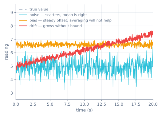
Noise, bias, and drift are different problems
- Noise varies randomly from sample to sample. Averaging or filtering reduces it.
- Bias is a fixed offset from the true value. Filtering will not remove it; you have to measure it during calibration and subtract it.
- Drift is a bias that changes slowly over time, usually with temperature. A calibration taken at startup gradually stops matching reality, which is why long runs need periodic recalibration or a reference to correct against.
Confusing these leads to the wrong fix—more filtering will never cure a bias.
Choosing a filter
Three common filters cover most cases:
- A moving average and an exponential low-pass both smooth random noise, trading responsiveness for smoothness through their window or time constant.
- A median filter is better at removing occasional spikes and dropouts, because a few bad samples do not move the middle value.
Pick the lightest filter that meets the requirement of whatever consumes the measurement—not the one that produces the smoothest-looking plot.
Filtering always adds lag
Every smoothing filter lags the true signal, and more smoothing means more lag. A low-pass filter with a long time constant rejects more noise but falls further behind fast changes. Always plot the filtered estimate against both the raw samples and the truth so the delay is visible before you put the filter inside a control loop, where lag can cause instability.
class LowPass:
    def __init__(self, alpha):
        self.alpha = alpha      # smaller alpha = smoother but more lag
        self.value = None
    def update(self, sample):
        if self.value is None:
            self.value = sample
        else:
            self.value += self.alpha * (sample - self.value)
        return self.value
What sensor fusion can and cannot do
Fusion combines several sensors into one estimate, and it helps only when the sensors contribute complementary information and their uncertainty is represented honestly. Combining two biased measurements does not create truth. A complementary filter, for example, trusts one sensor at high frequencies and another at low frequencies; a Kalman filter weights each source by its uncertainty. Either way, start with calibration, timestamps, and shared coordinate frames before fusing anything.
Timestamp everything
Samples rarely arrive at a perfectly fixed interval, and both filtering and fusion assume you know when each value was measured. Timestamps let you detect jitter, align data from different sensors, and reject stale readings. Log raw values beside processed ones so failures like clipping and dropouts stay reproducible.
Measure your sensor before you filter it
Choosing a filter before you know what the noise looks like is guessing. Ten minutes of logging settles it, and the procedure is the same for any sensor:
- Hold the sensor perfectly still against a known, unchanging input.
- Log a few thousand raw samples with timestamps.
- Compute the mean and the standard deviation.
- Plot the samples, and plot a histogram of them.
Those four numbers and two plots tell you which of the three faults you have:
| What you observe | What it is | The fix |
|---|---|---|
| Mean matches truth, values scatter symmetrically | Noise | Filter it |
| Mean is offset from truth, scatter is small | Bias | Measure and subtract it — filtering will never help |
| Mean walks away over minutes | Drift | Recalibrate periodically, or correct against a reference |
| Mostly tight, with occasional wild values | Outliers | Median, not an average |
| Values land on discrete steps | Quantisation | Expected; it bounds your resolution |
The histogram is the part people skip, and it is the most informative. Gaussian noise makes a bell; outliers make a bell with a few points far out in the tails. Those two need different filters, and no amount of staring at a time-series plot distinguishes them as clearly.
Choosing a filter, quantified
| Filter | Kills Gaussian noise | Kills outliers | Lag | Cost |
|---|---|---|---|---|
| Moving average, N samples | Yes — by √N | No — smears one spike over N samples | (N−1)/2 samples | N-sample buffer |
| Exponential low-pass (EMA) | Yes | No | ≈ (1−α)/α samples | One float |
| Median of N | Somewhat | Completely, up to N/2 outliers | (N−1)/2 samples | Sort, trivial at small N |
| Median then EMA | Yes | Yes | Both | Both |
The √N in the first row is the useful number: averaging 4 samples halves the noise; averaging 100 samples reduces it by ten, at the cost of 50 samples of lag. Noise reduction has sharply diminishing returns and lag does not, which is why very long averages are almost always the wrong answer.
For an EMA, the time constant relates to α by:
tau = dt x (1 - alpha) / alphaSo at a 10 ms loop, α = 0.1 gives a 90 ms time constant. Setting α by feel is how people end up with filters that are far slower than they realise — compute it once and you know what you have.
The lag is not free, and here is what it costs
Every smoothing filter delays the signal, and inside a control loop that delay is indistinguishable from the plant being slower to respond. It directly reduces how much gain the loop can tolerate before it oscillates.
| Filter | Lag at a 10 ms loop | Distance travelled at 0.3 m/s |
|---|---|---|
| Median of 3 | 10 ms | 3 mm |
| Median of 5 | 20 ms | 6 mm |
| Moving average of 10 | 45 ms | 14 mm |
| EMA, α = 0.1 | 90 ms | 27 mm |
| EMA, α = 0.02 | 490 ms | 147 mm |
That last row is worth sitting with. An α of 0.02 produces a beautifully smooth plot and half a second of lag — the robot is steering on where the obstacle was 15 cm ago. This is the single most common way a well-intentioned filter makes a robot worse, and it is invisible unless you plot filtered against raw with the truth alongside.
Pick the lightest filter that meets the requirement, and always check what the lag costs in the units the robot cares about — millimetres, or degrees, not samples.
A complementary filter, and how to choose its constant
The complementary filter is the workhorse of hobby robotics because it is three lines and it solves the real problem: two sensors that fail in opposite ways.
// gyroRate in deg/s, accelAngle in degrees, dt in seconds.
angle = alpha * (angle + gyroRate * dt) + (1.0f - alpha) * accelAngle;
alpha sets the crossover frequency — above it you trust the gyro, below it the
accelerometer:
tau = alpha x dt / (1 - alpha)          # the filter's time constant, seconds
f_crossover = 1 / (2 x pi x tau) # Hz| α at dt = 5 ms | Time constant | Crossover | Behaviour |
|---|---|---|---|
| 0.90 | 45 ms | 3.5 Hz | Very responsive, visibly noisy from the accelerometer |
| 0.98 | 245 ms | 0.65 Hz | The common default — a good balance |
| 0.995 | 1.0 s | 0.16 Hz | Very smooth, drifts noticeably before correcting |
| 0.999 | 5.0 s | 0.03 Hz | Effectively gyro-only over any short manoeuvre |
Choose it from the physics rather than by feel: the time constant should be long compared to the disturbances you want to reject, and short compared to the gyro’s drift rate. A gyro biased by 1 °/s reaches 1° of error in a second, so a time constant of several seconds lets real error accumulate before the accelerometer pulls it back.
Note also that α depends on dt. Copying an α from a project with a different loop rate gives
you a different filter — which is a common and invisible source of “these gains do not work
for me”.
What fusion cannot do
Fusion is not magic, and three limits are worth stating plainly:
It cannot remove a shared bias. Two accelerometers that both read 2° high produce a fused estimate that reads 2° high. Fusion exploits independent errors; a common-mode error survives untouched.
It cannot create information that is not there. No amount of filtering gives a six-axis IMU an absolute heading. Yaw has no gravity reference, so it drifts, and only a magnetometer or an external reference fixes it.
It cannot fix bad timestamps. Fusing a 10 Hz GPS fix with a 200 Hz gyro requires knowing when each was measured, to a fraction of the faster interval. A fix that is 100 ms stale and treated as current will actively corrupt an estimate the gyro alone had right.
Timestamps, concretely
“Timestamp everything” is easy to nod at and easy to skip. The practical version:
struct Sample {
  float value;
  unsigned long micros;    // when it was MEASURED, not when it was read
};

// Reject anything too old to be useful, rather than fusing it.
bool isFresh(const Sample &s, unsigned long maxAgeUs) {
  return (micros() - s.micros) < maxAgeUs;
}
Capture the timestamp as close to the measurement as possible — inside the interrupt, not after the parsing. A GPS sentence parsed 80 ms after the fix was taken and timestamped at parse time is 80 ms wrong, and nothing downstream can recover that.
Troubleshooting
| Symptom | Likely cause | Fix |
|---|---|---|
| More filtering, no improvement | It is bias, not noise | Measure the offset at rest and subtract |
| Estimate slowly walks away | Drift | Periodic recalibration, or an absolute reference |
| Occasional spike survives the filter | Using an average | Median rejects outliers; an average smears them |
| Control loop oscillates after adding a filter | Lag reduced the stable gain | Lighter filter, or retune |
| Smooth plot, robot reacts late | Time constant far longer than intended | Compute τ from α — do not set α by feel |
| Fused estimate worse than either sensor | Stale timestamps, or a shared bias | Timestamp at measurement; check both sensors’ offsets |
| Filter works on the bench, not on the robot | Vibration is a real signal, not noise | Soft-mount the sensor; the filter cannot tell them apart |
| Complementary filter behaves differently from a tutorial’s | α depends on dt |
Compute α for your loop rate |
Try it yourself
In the Robot Sensor Simulator you can dial in noise, bias, drift, and dropouts, then compare raw data against low-pass, moving-average, and median estimates. It is the quickest way to feel the noise-versus-lag trade-off—the same trade-off that decides how a robot reacts in the Obstacle Avoidance Simulator.
Explore the graph
Part of these builds
Projects and learning paths that include this tutorial.
Further reading