
Tutorial · Intermediate · 20 min read
Differential-Drive Odometry from Wheel Encoders
Calculate a differential-drive robot's position from left and right encoder motion, handle straight and curved travel, and measure odometry drift.
A differential-drive robot has two independently driven wheels separated by a track width. When both wheels move the same distance, the robot travels straight. When one travels farther, the chassis follows an arc. Odometry integrates those small motions over time to estimate pose: horizontal position x, vertical position y, and heading θ.
The estimate is local and cumulative. It starts from a chosen pose and cannot correct itself from wheel encoders alone. Small wheel-diameter, track-width, timing, and slip errors accumulate, so the goal is a useful short-term estimate with measured limits—not perfect ground truth.
Define one coordinate convention
Choose a frame before writing equations. A common two-dimensional convention is:
xpoints forward from the starting pose.ypoints left.- positive
θturns counter-clockwise. - left and right wheel distance are positive when the robot drives forward.
Store angles in radians internally. Convert to degrees only for display. Normalize heading if bounded values help debugging, but sine and cosine work with unbounded angles too.
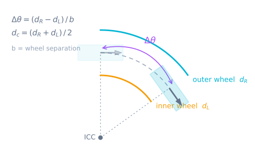
Let dL and dR be the left and right wheel distances since the previous update, and b the effective distance between the wheel contact lines.
Turn counts into metres
Everything above assumes you already have dL and dR in metres. Encoders do not produce metres; they produce counts. One conversion sits between them, and getting it wrong scales every number the rest of this page computes.
countsPerWheelTurn = PPR x edgesDecoded x gearRatio
metresPerCount     = (pi x wheelDiameter) / countsPerWheelTurn
edgesDecoded is 4 only if you decode both edges of both channels — the full quadrature. Decoding one channel’s rising edge gives 1, and it also throws away the direction information, so the robot cannot tell a reverse from a forward.
| Encoder and gearbox | Counts per wheel turn | Resolution on a 65 mm wheel |
|---|---|---|
| N20, 7 PPR magnetic, 100:1 | 2,800 | 73 um |
| N20, 7 PPR magnetic, 50:1 | 1,400 | 146 um |
| 11 PPR magnetic, 30:1 gearbox | 1,320 | 155 um |
| 20-slot optical disc, single channel, on the wheel | 20 | 10.2 mm |
The bottom row is the one that surprises people. A slotted disc zip-tied to the wheel is cheap, but 10 mm of quantisation means a 200 mm move is known to about 5%, and no amount of calibration recovers information the sensor never captured. The quadrature encoder tutorial covers the decoding side in full.
Resolution is a floor on precision, not a promise of accuracy. A 73 um count is meaningless if the wheel diameter is 2% wrong.
Calculate forward and angular motion
The center of the axle moves by the average wheel distance:
dCenter = (dR + dL) / 2
The heading changes according to their difference:
dTheta = (dR - dL) / b
Equal distances make dTheta = 0. Equal and opposite distances make dCenter = 0, so the robot rotates in place around the axle midpoint.
For small updates, applying translation at the midpoint heading is accurate and avoids a straight-line special case:
headingMid = theta + dTheta / 2
x = x + dCenter * cos(headingMid)
y = y + dCenter * sin(headingMid)
theta = theta + dTheta
This midpoint integration is simple enough for an embedded controller and behaves well when the loop runs frequently. An exact arc integration is useful for large steps, but it does not repair wrong wheel measurements.
Implement a repeatable update
Keep raw encoder totals and convert their differences to metres. Do not reset hardware counters on every loop; snapshots make rollover and diagnostics easier.
struct Pose { float x, y, theta; };

void updateOdometry(Pose& pose, float dLeft, float dRight, float trackWidth) {
  const float dCenter = 0.5f * (dLeft + dRight);
  const float dTheta = (dRight - dLeft) / trackWidth;
  const float headingMid = pose.theta + 0.5f * dTheta;

  pose.x += dCenter * cosf(headingMid);
  pose.y += dCenter * sinf(headingMid);
  pose.theta += dTheta;
}
Call this after atomically reading both encoders. The left and right snapshots should represent nearly the same instant; a long gap between them creates apparent steering during rapid motion.
If another subsystem needs velocity, divide the increments by the measured elapsed time. Pose integration itself uses distance, so loop-time jitter does not directly change the travelled distance estimate.
Read both encoders without losing counts
The function above is pure arithmetic. Feeding it correctly is where embedded odometry actually breaks, and three details carry almost all of the risk.
Snapshot both counters in the same instant. The interrupt handlers keep incrementing while your loop reads them. Reading left, doing some work, then reading right attributes motion that happened in between to one wheel only — which the equations faithfully interpret as a turn.
Never reset the hardware counters. Free-running totals plus a remembered previous value give you the delta, and they leave the raw count available for diagnostics.
Compute the delta in unsigned arithmetic. Signed overflow is undefined behaviour in C++; the cast dance below is defined, costs nothing, and stays correct across the wrap.
volatile int32_t leftCount = 0, rightCount = 0;   // written only by the ISRs

void isrLeft()  { leftCount  += digitalRead(L_CHAN_B) ? +1 : -1; }
void isrRight() { rightCount += digitalRead(R_CHAN_B) ? +1 : -1; }

constexpr float METRES_PER_COUNT = (3.14159265f * 0.065f) / 2800.0f;   // 72.9 um
constexpr float TRACK_WIDTH      = 0.152f;                             // calibrated, not measured

void odometryTick(Pose& pose) {
  int32_t nowLeft, nowRight;
  noInterrupts();                      // one instant, both wheels
  nowLeft  = leftCount;
  nowRight = rightCount;
  interrupts();

  static int32_t prevLeft = 0, prevRight = 0;
  // Unsigned subtraction wraps in a defined way; the cast back recovers the
  // signed delta even across the 2^32 boundary.
  const int32_t dLeftCounts  = (int32_t)((uint32_t)nowLeft  - (uint32_t)prevLeft);
  const int32_t dRightCounts = (int32_t)((uint32_t)nowRight - (uint32_t)prevRight);
  prevLeft  = nowLeft;
  prevRight = nowRight;

  updateOdometry(pose,
                 dLeftCounts  * METRES_PER_COUNT,
                 dRightCounts * METRES_PER_COUNT,
                 TRACK_WIDTH);
}
At 73 um per count a signed 32-bit counter wraps after about 157 km, so on a desk robot the wrap is theoretical. It costs two casts to be right about it anyway, and the same pattern is mandatory on a 16-bit counter, which wraps after 2.4 m.
Work through one turn
Suppose the left wheel moves 0.20 m, the right moves 0.30 m, and track width is 0.25 m:
dCenter = 0.25 mdTheta = (0.30 - 0.20) / 0.25 = 0.4 rad- from heading zero, midpoint heading is
0.2 rad dx ≈ 0.25 cos(0.2) = 0.245 mdy ≈ 0.25 sin(0.2) = 0.050 m
The robot ends slightly left of its original forward axis and rotated about 22.9°. Checking a hand calculation like this catches sign and unit errors before the code reaches hardware.
Calibrate the two dominant parameters
Effective wheel diameter controls distance scale. Drive a long measured straight line, compare reported and actual distance, and multiply the diameter scale by actual / reported. Calibrate each side if the robot curves despite equal commands.
Effective track width controls rotation scale. Command several full in-place rotations, measure actual heading change with an external reference, and adjust track width. Multiple turns magnify the error and make measurement easier. Tire scrub means the effective value may differ from ruler-measured wheel spacing.
Keep both parameters configurable. Surface, tire compression, payload, and wear can change them; hardware models need calibration knobs.
Know how fast the error grows
Calibration does not remove error, it shrinks the coefficient. Knowing the size of what is left tells you how long you can trust the estimate before something external has to correct it.
| Error source | Size of a realistic error | What it costs you |
|---|---|---|
| Wheel diameter scale | 1% | 10 cm over a 10 m straight run |
| Track width scale | 2% | 7.2 deg after one full rotation |
| Track width scale | 2% | 8.7 cm closure error on a 1 m square |
| Systematic wheel scrub | 2% per pivot | 0.9 deg per 90 deg turn, 45 deg after 50 turns |
| Random wheel scrub | 2% per pivot | about 6 deg after 50 turns, growing as the square root |
| Midpoint integration at 50 Hz | 0.04 rad per step at 2 rad/s | 0.007%, roughly 0.07 mm per metre |
The square figure comes from integrating a 1 m square with four in-place 90 deg turns and nothing wrong except the track width. Everything else is exact, and the robot still finishes 8.7 cm from where it started.
Read the last row against the first two. The integration maths is never your dominant error. It is three orders of magnitude below the calibration terms and four below slip, which is why raising the loop rate to chase precision is the wrong optimisation — and why the wheel slip page matters more to your final pose than anything on this page does.
Note also that systematic and random errors behave completely differently. A systematic scrub accumulates linearly and is worth calibrating out. A random one grows with the square root of the number of turns, so 50 turns costs about 6 deg rather than 45 — annoying, but not fixable by any amount of parameter tuning.
Choose an update rate
The arc between two samples is approximated by a straight chord at the midpoint heading, so the error depends on how much heading changes per step. For a step of dTheta radians the chord is short by roughly dTheta^2 / 24:
| Update rate | dTheta at 2 rad/s | Chord error | In practice |
|---|---|---|---|
| 200 Hz | 0.010 rad | 0.0004% | Pointless on this maths |
| 100 Hz | 0.020 rad | 0.002% | Free if the loop already runs here |
| 50 Hz | 0.040 rad | 0.007% | Comfortable default |
| 20 Hz | 0.100 rad | 0.04% | Fine for a slow indoor robot |
| 10 Hz | 0.200 rad | 0.17% | Visible on a fast spin |
| 5 Hz | 0.400 rad | 0.67% | Too slow to trust while turning |
Pick 50 Hz and stop thinking about it. Spend the attention you saved on synchronising the two encoder reads, which at any rate matters more than the rate itself: a 1 ms skew between the left and right snapshot while the wheels differ by 0.5 m/s invents 0.5 mm of wheel difference out of nothing, every single loop.
Add a gyro without confusing the frames
A gyro often provides a better short-term heading change than the difference between wheel encoders. You can use gyro heading for theta while still using average wheel distance for translation. Apply translation at the average of old and new gyro headings.
That does not make position absolute. Gyros have bias and wheel distance still slips. A global sensor—camera landmarks, lidar localization, or another external reference—is needed to correct accumulated pose.
In ROS terminology, a continuous local estimate belongs naturally in the odom frame. A localization system may update map → odom without forcing the locally smooth odom → base_link transform to jump.
Measure drift instead of hiding it
Run three repeatable tests:
- Drive forward and backward to the start.
- Rotate several turns and return to the original heading.
- Drive a large square and compare the final pose with the starting mark.
Log encoder deltas, computed pose, battery voltage, and surface. Repeat each test in both directions. Consistent scale error suggests calibration; error that changes with direction suggests backlash or asymmetry; error that changes by surface suggests slip.
Troubleshooting
| Symptom | Usually | Fix |
|---|---|---|
| Robot turns left, heading decreases | Sign or wheel order inverted | Swap it once, at the boundary where counts enter |
| Straight motion changes heading | Wheel scales differ, counts missed, or reads unsynchronised | Calibrate each side, then snapshot both counters together |
| Rotation consistently too large | Effective track width too small | Multiply track width by actual over commanded |
| Heading drifts only at speed | Interrupts being missed under load | Shorten the ISRs, or move decoding to hardware |
| Square never closes despite calibration | Slip and integration error accumulating | Add an external correction; no parameter fixes this |
| Position jumps after long runs | Counter rollover handled with signed arithmetic | Take the delta in unsigned, then cast back |
| Distance right, heading wrong | Track width uncalibrated, or a gyro fighting the encoders | Calibrate on rotations only, with distance already correct |
| Perfect in simulation, wrong on the floor | Model has no tyre deformation, backlash, or sensor timing | Trust the bench tests, not the simulator |
Try the steering consequences in the Line Follower Simulator and compare local motion estimates with the mapping concepts in SLAM fundamentals. For the task that depends on this estimate most directly — driving parallel rows across a whole floor — see coverage path planning and the coverage simulator.
Explore the graph
Part of these builds
Projects and learning paths that include this tutorial.
- ProjectBuild a GPS Waypoint Rover That Drives Itself
- ProjectBuild a Line Follower Robot: From Simulator to Real Track
- ProjectBuild a Micromouse: A Flood-Fill Maze-Solving Robot
- ProjectBuild a Room Coverage Robot That Sweeps a Floor
- ProjectBuild an Obstacle-Avoiding Robot: Sense, Scan, and Steer
- Learning pathMotor Control for Robots: A Learning Roadmap
- Learning pathPath Following for Robots: A Learning Roadmap
Further reading