
Tutorial · Advanced · 22 min read
Inverse Kinematics of a Two-Link Robot Arm
Understand inverse kinematics for a planar two-link arm: elbow-up and elbow-down solutions, the reachable workspace, singularities, and unreachable targets.
Forward kinematics is easy: given the joint angles, multiply the link transforms and you know where the tool is. Inverse kinematics runs the other way—given a target position, find joint angles that reach it—and that direction is where the interesting problems live. A planar two-link arm is the smallest example that shows all of them. Explore it in the Robot Arm Simulator.
The reachable workspace
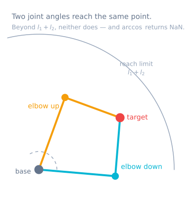
With link lengths L₁ and L₂, the tool can only reach points inside an annulus (a ring). The outer radius is L₁ + L₂ (arm fully stretched) and the inner radius is |L₁ − L₂| (arm fully folded). Anything outside the ring is too far; anything inside the hole is too close. No joint angles can reach those points, so the correct answer is simply “unreachable.”
Two solutions: elbow-up and elbow-down
For most targets inside the ring, the elbow can bend two ways and still place the tool on the same point. These are the elbow-up and elbow-down configurations. They come from a ± in the law-of-cosines angle for the second joint:
cos(θ₂) = (x² + y² − L₁² − L₂²) / (2·L₁·L₂)
θ₂ = ± acos(cos(θ₂))        # + is one elbow, − is the other
θ₁ = atan2(y, x) − atan2(L₂·sin θ₂, L₁ + L₂·cos θ₂)
Because there are two valid answers, inverse kinematics is not a single function—it is a choice. Robots pick the configuration that keeps joints away from their limits, minimizes movement from the current pose, or avoids an obstacle.
Singularities
At the edges of the workspace—arm fully stretched or fully folded—the two solutions merge into one. These are singularities, and near them a small motion of the tool can demand a huge motion of the joints. Planners slow down or route around singular poses because the arm briefly loses the ability to move the tool in one direction.
When is there no solution?
A target has no solution when it falls outside the reachable ring, when it would require a joint angle the hardware forbids, or when it demands an orientation the available joints cannot produce. A good simulator distinguishes these cases honestly instead of snapping to the nearest pose and pretending it succeeded.
Analytic versus numerical solvers
For two or three links the geometry has a closed-form (analytic) solution, so you compute the joint angles directly, exactly, and fast. That makes analytic IK ideal for teaching and for testing. Redundant or fully spatial arms usually have no closed form and need numerical solvers that iterate toward a solution—more general, but slower and harder to reason about because they can miss solutions or stall near singularities.
The solver, written safely
The equations above are correct and will still produce NaN on real hardware. Here is the same maths with every failure handled explicitly:
enum IkStatus { IK_OK, IK_TOO_FAR, IK_TOO_CLOSE, IK_JOINT_LIMIT, IK_SINGULAR };

struct IkResult {
  IkStatus status;
  float theta1, theta2;      // radians
};

IkResult solveIk(float x, float y, float L1, float L2, bool elbowUp) {
  IkResult r{};

  const float r2 = x * x + y * y;
  const float reach = sqrtf(r2);

  // 1. Reachability FIRST, before any trigonometry.
  //    A small epsilon keeps a target exactly on the boundary from
  //    producing an acos argument of 1.0000001 through rounding.
  const float eps = 1e-4f;
  if (reach > L1 + L2 - eps)          { r.status = IK_TOO_FAR;   return r; }
  if (reach < fabsf(L1 - L2) + eps)   { r.status = IK_TOO_CLOSE; return r; }

  // 2. Now acos is guaranteed to be in range.
  float c2 = (r2 - L1 * L1 - L2 * L2) / (2.0f * L1 * L2);
  c2 = constrain(c2, -1.0f, 1.0f);              // belt and braces
  const float s2 = sqrtf(1.0f - c2 * c2);

  r.theta2 = elbowUp ? atan2f(s2, c2) : atan2f(-s2, c2);

  // 3. atan2, never atan — this is what gets all four quadrants right.
  r.theta1 = atan2f(y, x) - atan2f(L2 * sinf(r.theta2), L1 + L2 * cosf(r.theta2));

  // 4. Warn near the boundary, where the arm is ill-conditioned.
  if (reach > (L1 + L2) * 0.95f) { r.status = IK_SINGULAR; return r; }

  // 5. Mechanical limits are part of the answer, not an afterthought.
  if (r.theta1 < T1_MIN || r.theta1 > T1_MAX ||
      r.theta2 < T2_MIN || r.theta2 > T2_MAX) { r.status = IK_JOINT_LIMIT; return r; }

  r.status = IK_OK;
  return r;
}
Five details separate this from the textbook version, and each corresponds to a real failure:
Reachability before trigonometry. If the target is beyond L1 + L2, the cosine rule
produces an argument outside −1 to 1 and acos returns NaN. That NaN then flows into the servo
command as a garbage angle — which is why an unreachable target so often produces a violent
movement rather than a refusal to move.
The epsilon. A target computed to sit exactly on the boundary can, after floating-point
rounding, give c2 = 1.0000001. Testing reachability with a small margin catches it before
acos does.
atan2f, not atan. Plain atan takes a single quotient and cannot distinguish a target
in front from its mirror behind, so the arm works in two quadrants and mirrors in the other
two. This is the single most common bug in a first IK implementation.
A singularity warning rather than a refusal. Near full extension the solution is still valid but ill-conditioned — a small tool motion demands an enormous joint motion. Flagging it lets the caller slow down or route around it.
Joint limits as a status. An arm whose shoulder cannot go below −10° has targets that are geometrically reachable and mechanically not. Clamping silently produces an arm that goes somewhere near the target and reports success.
Choosing between the two solutions
The maths gives you both branches and cannot tell you which to use. That is a robotics decision, and there are four common rules:
| Rule | Choose the branch that… | Good for |
|---|---|---|
| Minimum motion | Is closest to the current joint angles | Smooth continuous paths — the usual default |
| Fixed branch | Is always elbow-up (or always down) | Predictability; avoiding a table below the arm |
| Joint-limit margin | Keeps both joints furthest from their limits | Arms with restricted travel |
| Obstacle avoidance | Does not collide with a known obstacle | Cluttered workspaces |
Minimum motion is the right default, and the reason is what happens without it: if the solver silently switches branch partway along a path, the arm flips through a large, fast, completely unplanned motion. On a real arm that is alarming and can be destructive.
// Pick the branch closest to where the arm already is.
IkResult up   = solveIk(x, y, L1, L2, true);
IkResult down = solveIk(x, y, L1, L2, false);

if (up.status == IK_OK && down.status == IK_OK) {
  const float costUp   = fabsf(up.theta1   - cur1) + fabsf(up.theta2   - cur2);
  const float costDown = fabsf(down.theta1 - cur1) + fabsf(down.theta2 - cur2);
  return (costUp <= costDown) ? up : down;
}
return (up.status == IK_OK) ? up : down;
Straight lines need IK at every step
Interpolating between two poses in joint space — moving each joint linearly from its start angle to its end angle — is simple and makes the tool follow a curve. For many tasks that is fine. For anything that has to travel in a straight line, you interpolate in Cartesian space and solve IK at every step:
void moveStraight(float x0, float y0, float x1, float y1, int steps) {
  for (int i = 1; i <= steps; i++) {
    const float t = (float)i / steps;
    const float x = x0 + (x1 - x0) * t;
    const float y = y0 + (y1 - y0) * t;

    IkResult r = solveClosest(x, y);
    if (r.status != IK_OK) { abortMove(r.status); return; }   // do not skip the point
    commandJoints(r.theta1, r.theta2);
  }
}
Two things become visible the first time you do this. Joint velocity is not constant even though the tool speed is — near the workspace edge the joints have to move much faster for the same tool motion. And a straight line can pass through a region the arm cannot reach even when both endpoints are fine, which is why the status check inside the loop matters rather than just at the ends.
From joint angles to servo counts
The solver returns joint angles in a mathematical frame. A servo knows nothing about that frame: its zero is wherever the horn was fitted, and it may rotate the opposite way.
struct Joint {
  uint8_t channel;
  float   offsetDeg;   // servo angle when the joint is at mathematical zero
  int8_t  sign;        // +1 or -1
  float   minDeg, maxDeg;
};

int servoAngle(const Joint &j, float jointRad) {
  const float deg = jointRad * 57.2957795f;
  const float clamped = constrain(deg, j.minDeg, j.maxDeg);
  return (int)(j.offsetDeg + j.sign * clamped);
}
That struct is the entire bridge between the kinematics and the hardware, and keeping it explicit is what makes it possible to tell a solver bug from a calibration one. An arm that moves smoothly and lands nowhere near the target is almost always this, not the maths.
Troubleshooting
| Symptom | Likely cause | Fix |
|---|---|---|
| Reaches correctly in front, mirrors behind | atan instead of atan2 |
atan2 resolves all four quadrants |
| Returns NaN, arm lunges | acos argument out of range |
Test reachability before the trigonometry |
| Targets near the base fail | Inside the |L1 − L2| hole |
Correct — the workspace is an annulus, not a disc |
| Arm flips violently mid-path | Solver switched branch | Choose the branch closest to the current pose |
| Joint velocity spikes near full extension | Singularity | Keep planned paths inside ~95% of maximum reach |
| Round-trips correctly, lands in the wrong place | Servo offset or sign | Calibrate each joint’s offset and direction |
| Consistently short at full reach | Gravity sag, not maths | Check the shoulder torque budget; counterbalance |
| Lands differently depending on approach | Gearbox backlash | Always approach a target from the same direction |
| Straight-line move fails partway | Path leaves the workspace between the endpoints | Check status at every interpolation step |
Try it yourself
In the Robot Arm Simulator, drag the target around and watch the arm solve for it in real time. Toggle the elbow branch to see the alternate solution, push the target outside the ring to see an honest “unreachable,” and move toward the workspace edge to feel a singularity.
Explore the graph
Part of these builds
Projects and learning paths that include this tutorial.
Further reading